


Note
Click here to download the full example code
Spatial Transformer Networks Tutorial
Created On: Nov 08, 2017 | Last Updated: Jan 19, 2024 | Last Verified: Nov 05, 2024
Author: Ghassen HAMROUNI

In this tutorial, you will learn how to augment your network using a visual attention mechanism called spatial transformer networks. You can read more about the spatial transformer networks in the DeepMind paper
Spatial transformer networks are a generalization of differentiable attention to any spatial transformation. Spatial transformer networks (STN for short) allow a neural network to learn how to perform spatial transformations on the input image in order to enhance the geometric invariance of the model. For example, it can crop a region of interest, scale and correct the orientation of an image. It can be a useful mechanism because CNNs are not invariant to rotation and scale and more general affine transformations.
One of the best things about STN is the ability to simply plug it into any existing CNN with very little modification.
# License: BSD
# Author: Ghassen Hamrouni

import torch
import torch.nn as nn
import torch.nn.functional as F
import torch.optim as optim
import torchvision
from torchvision import datasets, transforms
import matplotlib.pyplot as plt
import numpy as np

plt.ion()   # interactive mode
<contextlib.ExitStack object at 0x7f86efde6f20>
Loading the data
In this post we experiment with the classic MNIST dataset. Using a standard convolutional network augmented with a spatial transformer network.
from six.moves import urllib
opener = urllib.request.build_opener()
opener.addheaders = [('User-agent', 'Mozilla/5.0')]
urllib.request.install_opener(opener)

device = torch.device("cuda" if torch.cuda.is_available() else "cpu")

# Training dataset
train_loader = torch.utils.data.DataLoader(
    datasets.MNIST(root='.', train=True, download=True,
                   transform=transforms.Compose([
                       transforms.ToTensor(),
                       transforms.Normalize((0.1307,), (0.3081,))
                   ])), batch_size=64, shuffle=True, num_workers=4)
# Test dataset
test_loader = torch.utils.data.DataLoader(
    datasets.MNIST(root='.', train=False, transform=transforms.Compose([
        transforms.ToTensor(),
        transforms.Normalize((0.1307,), (0.3081,))
    ])), batch_size=64, shuffle=True, num_workers=4)
  0%|          | 0.00/9.91M [00:00<?, ?B/s]
100%|##########| 9.91M/9.91M [00:00<00:00, 136MB/s]

  0%|          | 0.00/28.9k [00:00<?, ?B/s]
100%|##########| 28.9k/28.9k [00:00<00:00, 25.3MB/s]

  0%|          | 0.00/1.65M [00:00<?, ?B/s]
100%|##########| 1.65M/1.65M [00:00<00:00, 184MB/s]

  0%|          | 0.00/4.54k [00:00<?, ?B/s]
100%|##########| 4.54k/4.54k [00:00<00:00, 20.7MB/s]
Depicting spatial transformer networks
Spatial transformer networks boils down to three main components :
The localization network is a regular CNN which regresses the transformation parameters. The transformation is never learned explicitly from this dataset, instead the network learns automatically the spatial transformations that enhances the global accuracy.
The grid generator generates a grid of coordinates in the input image corresponding to each pixel from the output image.
The sampler uses the parameters of the transformation and applies it to the input image.

Note
We need the latest version of PyTorch that contains affine_grid and grid_sample modules.
class Net(nn.Module):
    def __init__(self):
        super(Net, self).__init__()
        self.conv1 = nn.Conv2d(1, 10, kernel_size=5)
        self.conv2 = nn.Conv2d(10, 20, kernel_size=5)
        self.conv2_drop = nn.Dropout2d()
        self.fc1 = nn.Linear(320, 50)
        self.fc2 = nn.Linear(50, 10)

        # Spatial transformer localization-network
        self.localization = nn.Sequential(
            nn.Conv2d(1, 8, kernel_size=7),
            nn.MaxPool2d(2, stride=2),
            nn.ReLU(True),
            nn.Conv2d(8, 10, kernel_size=5),
            nn.MaxPool2d(2, stride=2),
            nn.ReLU(True)
        )

        # Regressor for the 3 * 2 affine matrix
        self.fc_loc = nn.Sequential(
            nn.Linear(10 * 3 * 3, 32),
            nn.ReLU(True),
            nn.Linear(32, 3 * 2)
        )

        # Initialize the weights/bias with identity transformation
        self.fc_loc[2].weight.data.zero_()
        self.fc_loc[2].bias.data.copy_(torch.tensor([1, 0, 0, 0, 1, 0], dtype=torch.float))

    # Spatial transformer network forward function
    def stn(self, x):
        xs = self.localization(x)
        xs = xs.view(-1, 10 * 3 * 3)
        theta = self.fc_loc(xs)
        theta = theta.view(-1, 2, 3)

        grid = F.affine_grid(theta, x.size())
        x = F.grid_sample(x, grid)

        return x

    def forward(self, x):
        # transform the input
        x = self.stn(x)

        # Perform the usual forward pass
        x = F.relu(F.max_pool2d(self.conv1(x), 2))
        x = F.relu(F.max_pool2d(self.conv2_drop(self.conv2(x)), 2))
        x = x.view(-1, 320)
        x = F.relu(self.fc1(x))
        x = F.dropout(x, training=self.training)
        x = self.fc2(x)
        return F.log_softmax(x, dim=1)


model = Net().to(device)
Training the model
Now, let’s use the SGD algorithm to train the model. The network is learning the classification task in a supervised way. In the same time the model is learning STN automatically in an end-to-end fashion.
optimizer = optim.SGD(model.parameters(), lr=0.01)


def train(epoch):
    model.train()
    for batch_idx, (data, target) in enumerate(train_loader):
        data, target = data.to(device), target.to(device)

        optimizer.zero_grad()
        output = model(data)
        loss = F.nll_loss(output, target)
        loss.backward()
        optimizer.step()
        if batch_idx % 500 == 0:
            print('Train Epoch: {} [{}/{} ({:.0f}%)]\tLoss: {:.6f}'.format(
                epoch, batch_idx * len(data), len(train_loader.dataset),
                100. * batch_idx / len(train_loader), loss.item()))
#
# A simple test procedure to measure the STN performances on MNIST.
#


def test():
    with torch.no_grad():
        model.eval()
        test_loss = 0
        correct = 0
        for data, target in test_loader:
            data, target = data.to(device), target.to(device)
            output = model(data)

            # sum up batch loss
            test_loss += F.nll_loss(output, target, size_average=False).item()
            # get the index of the max log-probability
            pred = output.max(1, keepdim=True)[1]
            correct += pred.eq(target.view_as(pred)).sum().item()

        test_loss /= len(test_loader.dataset)
        print('\nTest set: Average loss: {:.4f}, Accuracy: {}/{} ({:.0f}%)\n'
              .format(test_loss, correct, len(test_loader.dataset),
                      100. * correct / len(test_loader.dataset)))
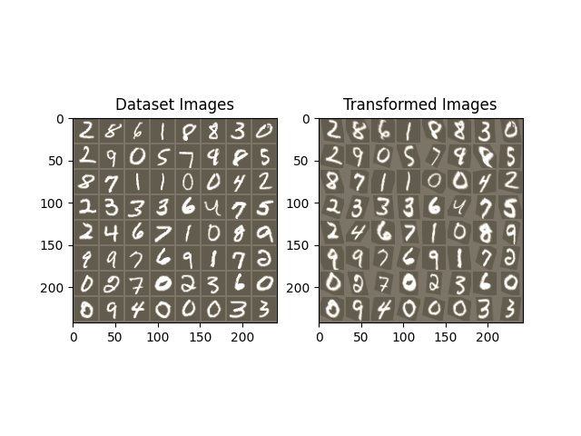
Visualizing the STN results
Now, we will inspect the results of our learned visual attention mechanism.
We define a small helper function in order to visualize the transformations while training.
def convert_image_np(inp):
    """Convert a Tensor to numpy image."""
    inp = inp.numpy().transpose((1, 2, 0))
    mean = np.array([0.485, 0.456, 0.406])
    std = np.array([0.229, 0.224, 0.225])
    inp = std * inp + mean
    inp = np.clip(inp, 0, 1)
    return inp

# We want to visualize the output of the spatial transformers layer
# after the training, we visualize a batch of input images and
# the corresponding transformed batch using STN.


def visualize_stn():
    with torch.no_grad():
        # Get a batch of training data
        data = next(iter(test_loader))[0].to(device)

        input_tensor = data.cpu()
        transformed_input_tensor = model.stn(data).cpu()

        in_grid = convert_image_np(
            torchvision.utils.make_grid(input_tensor))

        out_grid = convert_image_np(
            torchvision.utils.make_grid(transformed_input_tensor))

        # Plot the results side-by-side
        f, axarr = plt.subplots(1, 2)
        axarr[0].imshow(in_grid)
        axarr[0].set_title('Dataset Images')

        axarr[1].imshow(out_grid)
        axarr[1].set_title('Transformed Images')

for epoch in range(1, 20 + 1):
    train(epoch)
    test()

# Visualize the STN transformation on some input batch
visualize_stn()

plt.ioff()
plt.show()
/usr/local/lib/python3.10/dist-packages/torch/nn/functional.py:5082: UserWarning:

Default grid_sample and affine_grid behavior has changed to align_corners=False since 1.3.0. Please specify align_corners=True if the old behavior is desired. See the documentation of grid_sample for details.

/usr/local/lib/python3.10/dist-packages/torch/nn/functional.py:5015: UserWarning:

Default grid_sample and affine_grid behavior has changed to align_corners=False since 1.3.0. Please specify align_corners=True if the old behavior is desired. See the documentation of grid_sample for details.

Train Epoch: 1 [0/60000 (0%)]   Loss: 2.320278
Train Epoch: 1 [32000/60000 (53%)]      Loss: 0.635376
/usr/local/lib/python3.10/dist-packages/torch/nn/_reduction.py:51: UserWarning:

size_average and reduce args will be deprecated, please use reduction='sum' instead.


Test set: Average loss: 0.2449, Accuracy: 9296/10000 (93%)

Train Epoch: 2 [0/60000 (0%)]   Loss: 0.593936
Train Epoch: 2 [32000/60000 (53%)]      Loss: 0.182897

Test set: Average loss: 0.1405, Accuracy: 9538/10000 (95%)

Train Epoch: 3 [0/60000 (0%)]   Loss: 0.265780
Train Epoch: 3 [32000/60000 (53%)]      Loss: 0.185509

Test set: Average loss: 0.1370, Accuracy: 9545/10000 (95%)

Train Epoch: 4 [0/60000 (0%)]   Loss: 0.460517
Train Epoch: 4 [32000/60000 (53%)]      Loss: 0.133166

Test set: Average loss: 0.0966, Accuracy: 9706/10000 (97%)

Train Epoch: 5 [0/60000 (0%)]   Loss: 0.254712
Train Epoch: 5 [32000/60000 (53%)]      Loss: 0.309164

Test set: Average loss: 0.0777, Accuracy: 9751/10000 (98%)

Train Epoch: 6 [0/60000 (0%)]   Loss: 0.137199
Train Epoch: 6 [32000/60000 (53%)]      Loss: 0.312439

Test set: Average loss: 0.0664, Accuracy: 9798/10000 (98%)

Train Epoch: 7 [0/60000 (0%)]   Loss: 0.161752
Train Epoch: 7 [32000/60000 (53%)]      Loss: 0.280732

Test set: Average loss: 0.0639, Accuracy: 9803/10000 (98%)

Train Epoch: 8 [0/60000 (0%)]   Loss: 0.089810
Train Epoch: 8 [32000/60000 (53%)]      Loss: 0.108901

Test set: Average loss: 0.0765, Accuracy: 9779/10000 (98%)

Train Epoch: 9 [0/60000 (0%)]   Loss: 0.104590
Train Epoch: 9 [32000/60000 (53%)]      Loss: 0.111533

Test set: Average loss: 0.0612, Accuracy: 9801/10000 (98%)

Train Epoch: 10 [0/60000 (0%)]  Loss: 0.178695
Train Epoch: 10 [32000/60000 (53%)]     Loss: 0.049960

Test set: Average loss: 0.0543, Accuracy: 9827/10000 (98%)

Train Epoch: 11 [0/60000 (0%)]  Loss: 0.143058
Train Epoch: 11 [32000/60000 (53%)]     Loss: 0.399670

Test set: Average loss: 0.0465, Accuracy: 9847/10000 (98%)

Train Epoch: 12 [0/60000 (0%)]  Loss: 0.080671
Train Epoch: 12 [32000/60000 (53%)]     Loss: 0.369977

Test set: Average loss: 0.0515, Accuracy: 9850/10000 (98%)

Train Epoch: 13 [0/60000 (0%)]  Loss: 0.198029
Train Epoch: 13 [32000/60000 (53%)]     Loss: 0.093692

Test set: Average loss: 0.0441, Accuracy: 9878/10000 (99%)

Train Epoch: 14 [0/60000 (0%)]  Loss: 0.113596
Train Epoch: 14 [32000/60000 (53%)]     Loss: 0.088270

Test set: Average loss: 0.0950, Accuracy: 9707/10000 (97%)

Train Epoch: 15 [0/60000 (0%)]  Loss: 0.178823
Train Epoch: 15 [32000/60000 (53%)]     Loss: 0.052203

Test set: Average loss: 0.0394, Accuracy: 9885/10000 (99%)

Train Epoch: 16 [0/60000 (0%)]  Loss: 0.136575
Train Epoch: 16 [32000/60000 (53%)]     Loss: 0.149104

Test set: Average loss: 0.0449, Accuracy: 9867/10000 (99%)

Train Epoch: 17 [0/60000 (0%)]  Loss: 0.266379
Train Epoch: 17 [32000/60000 (53%)]     Loss: 0.063003

Test set: Average loss: 0.0389, Accuracy: 9884/10000 (99%)

Train Epoch: 18 [0/60000 (0%)]  Loss: 0.061570
Train Epoch: 18 [32000/60000 (53%)]     Loss: 0.190108

Test set: Average loss: 0.0435, Accuracy: 9865/10000 (99%)

Train Epoch: 19 [0/60000 (0%)]  Loss: 0.154054
Train Epoch: 19 [32000/60000 (53%)]     Loss: 0.024179

Test set: Average loss: 0.0535, Accuracy: 9847/10000 (98%)

Train Epoch: 20 [0/60000 (0%)]  Loss: 0.052457
Train Epoch: 20 [32000/60000 (53%)]     Loss: 0.141707

Test set: Average loss: 0.0450, Accuracy: 9884/10000 (99%)
Total running time of the script: ( 1 minutes 36.039 seconds)
